Patch Filtering

Patch filtering is useful if your data contains large areas with no signal. These areas can be filtered from the training process which can speed up the convergence of the model.

How does it work?

CAREamics will perform a first pass through all the data before training starts to determine regions of background and regions of signal. Background regions will not be completely be excluded from training, instead their probability of being selected during an epoch will be reduced.

There are two options for the filtering function, either:

• pre-computed masks can be provided, or
• one of the built-in filtering functions can be selected and parametrized.

Pre-computed masks

Using precomputed masks is relatively simple, the masks in the same format as the data — either as an array or saved in files — can be provided during training.

careamist.train(
    train_data=train_data,
    filtering_mask=mask_data,  # (1)!
)

careamist.train(
    train_data=train_data,
    train_data_target=train_target,
    filtering_mask=mask_data,  # (1)!
)

Filtering functions

CAREamics has 3 built-in filtering functions, which work by filtering out patches using thresholds on different metrics:

• MaxPatchFilter: that filters the data based on the max value of each region.
• MeanStdPatchFilter: that filters the data based on the mean and optionally the standard deviation of regions of the data.
• ShannonPatchFilter: that filters the data based on the shannon entropy of regions of the data.

Finding appropriate thresholds

Finding appropriate thresholds requires manually inspecting some examples. The patch filter classes provide filter_map and plot_filter_map which can be used to visualize at what threshold a region will be considered background.

For demonstration purposes we will use the Hagen dataset which is used in other CAREamics examples; however, it doesn't have enough background area to typically require patch filtering.

from pathlib import Path

import matplotlib.pyplot as plt
import pooch
import tifffile

from careamics.dataset.patch_filter import (
    MaxPatchFilter,
    MeanStdPatchFilter,
    ShannonPatchFilter,
)

# --- download the data
# folder in which to save all the data
root = Path("hagen")

# download the data using pooch
data_root = root / "data"
dataset_url = "https://zenodo.org/records/10925855/files/noisy.tiff?download=1"

file = pooch.retrieve(
    url=dataset_url,
    known_hash="ff12ee5566f443d58976757c037ecef8bf53a00794fa822fe7bcd0dd776a9c0f",
    path=data_root,
)

# Shape: (79, 1024, 1024), axes: SYX
img = tifffile.imread(file)

Now we inspect the filter maps to decide on a patch filtering function and threshold. For data with multiple samples it is generally a good idea to inspect the filter maps of a few different samples; and for 3D data one should look at multiple z-slices.

sample_idx = 4

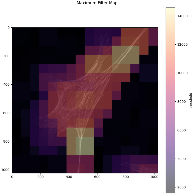
max_filter_map = MaxPatchFilter.filter_map(img[sample_idx], (64, 64))
MaxPatchFilter.plot_filter_map(img[sample_idx], max_filter_map)

shannon_filter_map = ShannonPatchFilter.filter_map(img[sample_idx], (64, 64))
ShannonPatchFilter.plot_filter_map(img[sample_idx], shannon_filter_map)

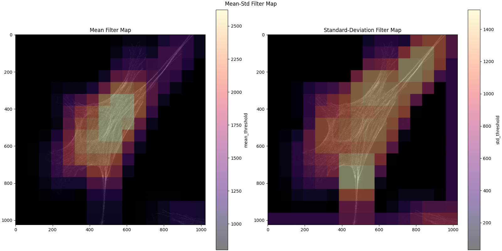
meanstd_filter_map = MeanStdPatchFilter.filter_map(img[sample_idx], (64, 64))
MeanStdPatchFilter.plot_filter_map(img[sample_idx], meanstd_filter_map)

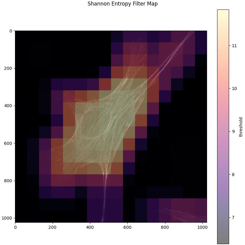
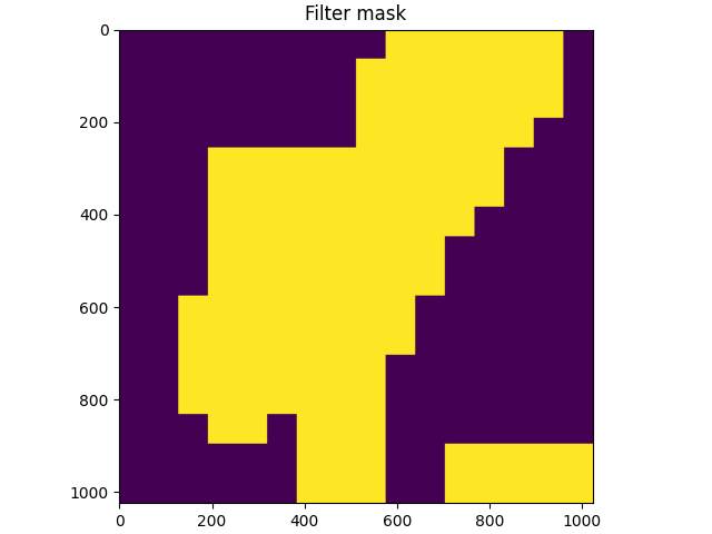
We will choose the shannon patch filter, with a threshold of 7.5, and to confirm that this is a good choice we will look at the resulting mask, by using the ShannonPatchFilter.apply_filter method.

plt.figure(constrained_layout=True)
plt.imshow(ShannonPatchFilter.apply_filter(shannon_filter_map, threshold=7.5))
plt.title("Filter mask")

Training

Next, we have to build the configuration.

Each of the patch filter classes has a corresponding configuration class, where the threshold parameters can be set:

• MaxPatchFilterConfig
• MeanStdPatchFilterConfig
• ShannonPatchFilterConfig

We will create the configuration using create_advanced_n2v_config and passing ShannonPatchFilterConfig with our selected threshold to the patch_filter_config argument.

from careamics import CAREamist
from careamics.config import ShannonPatchFilterConfig, create_advanced_n2v_config

config = create_advanced_n2v_config(
    "hagen-shannon-filtering",
    data_type="array",
    axes="SYX",
    patch_size=(64, 64),
    batch_size=64,
    num_epochs=10,
    patch_filter_config=ShannonPatchFilterConfig(threshold=7.5),  # (1)!
)

careamist = CAREamist(config=config)
careamist.train(train_data=img)

1. Using shannon filtering with a threshold of 7.5

Filtering background patches with filtering function shannon: 100%|██████████| 79/79 [00:06<00:00, 12.79it/s]
Found 6345 background regions. Number of patches has been reduced to 14553 from 20224.